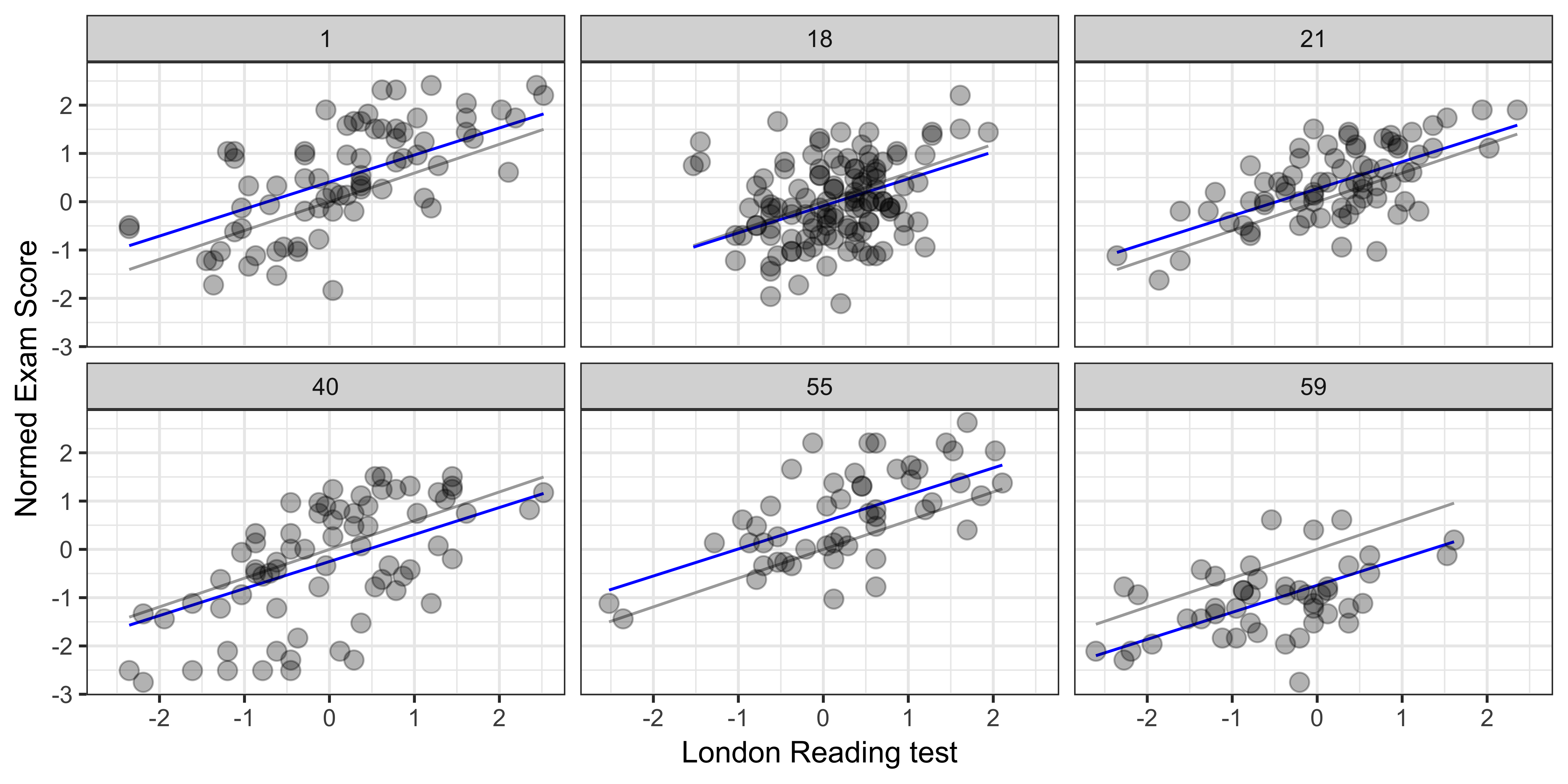
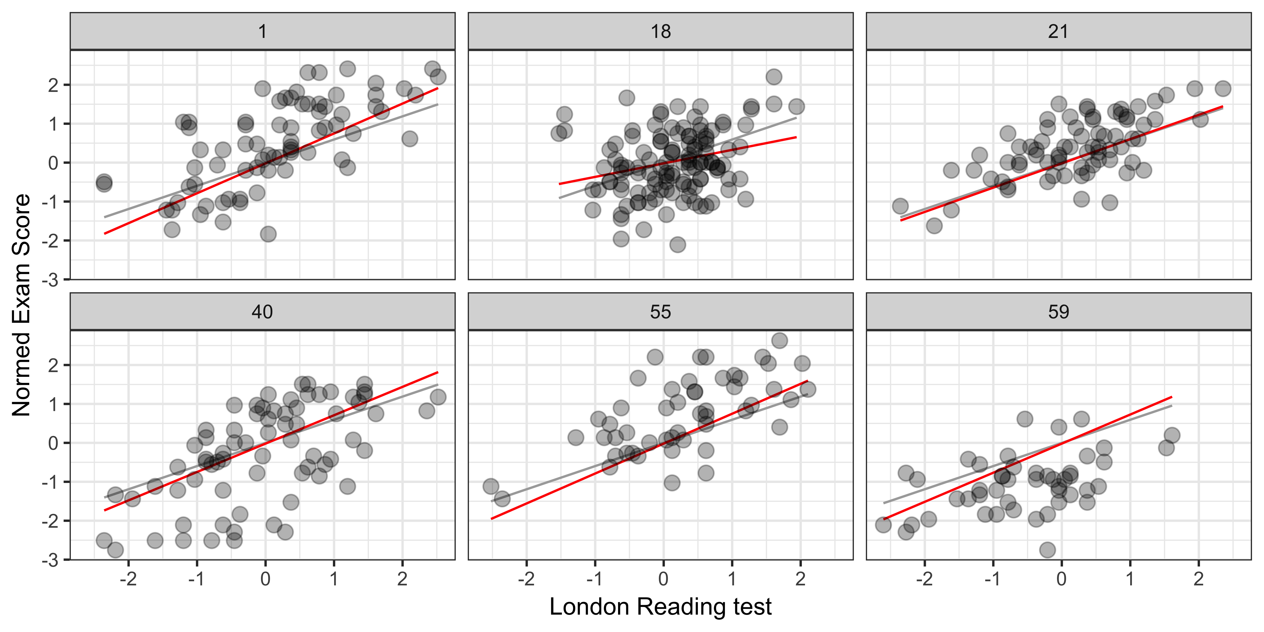
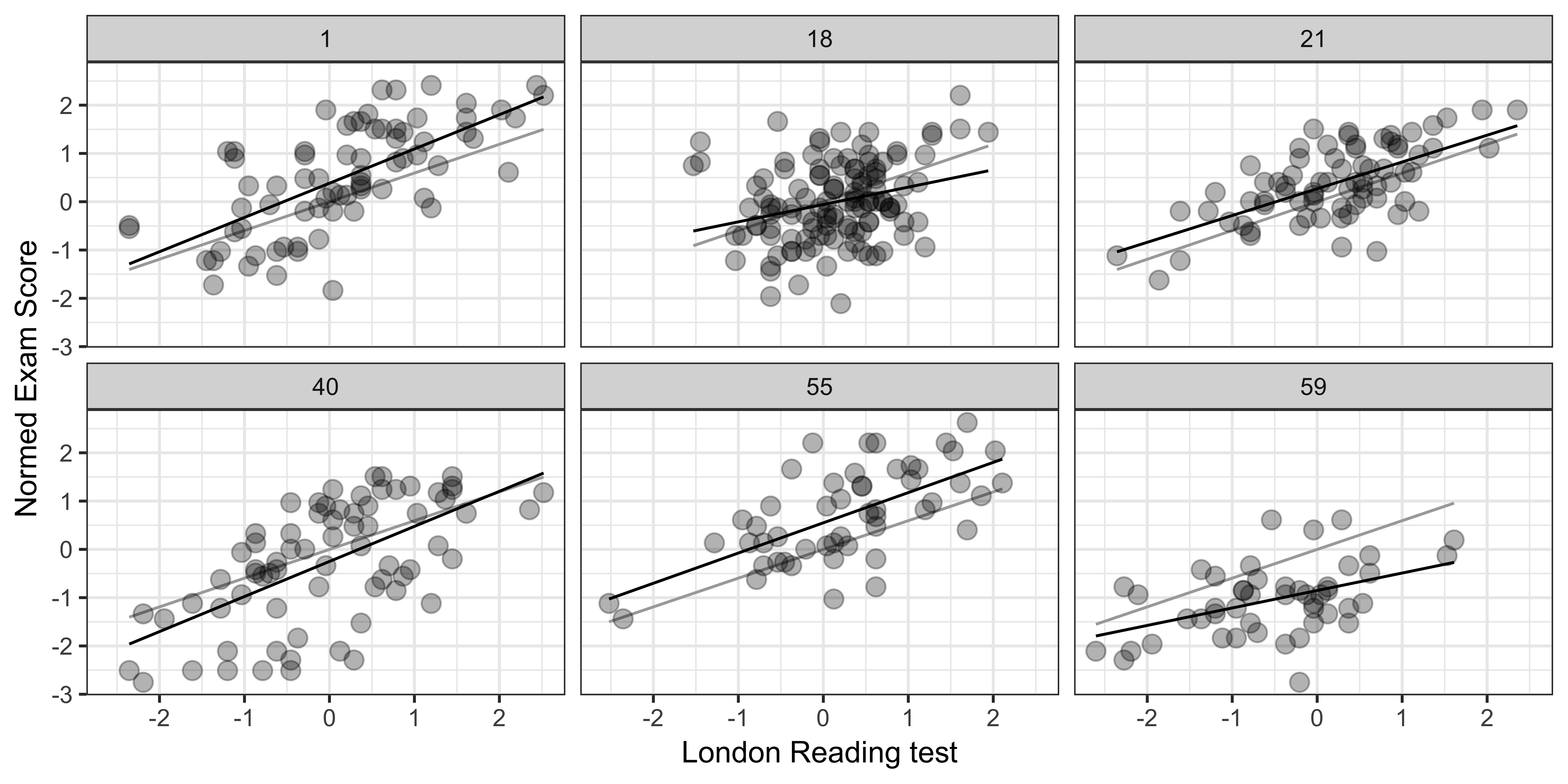
Lecture 11: PY 0782 - Advanced Quantitative Research Methods

class: center, middle, inverse, title-slide

# Lecture 11: PY 0782 - Advanced Quantitative Research Methods
### Dr. Thomas Pollet, Northumbria University (<a href="mailto:thomas.pollet@northumbria.ac.uk">thomas.pollet@northumbria.ac.uk</a>)
### 2018-12-16 | <a href="http://tvpollet.github.io/disclaimer">disclaimer</a>

---

## PY0782: Advanced Quantitative research methods.

* Last lecture:  Multilevel: part I.

* Today: Multilevel: part II.

I solved something for this lecture, remember those overflowing code bits, meet ['xaringan'](https://github.com/yihui/xaringan)

---

## Reload the data.

```r
setwd("~/Dropbox/Teaching_MRes_Northumbria/Lecture11")
library(mlmRev) # contains data
library(lme4)
Exam<-mlmRev::Exam
fixed_pred<-lmer(normexam ~ standLRT + (1 | school), data=Exam, REML=F)
```

---
## Make a plot

```r
library(ggplot2)
library(dplyr)
#subset 3 schools (just picked 3 from the dataframe)
subset<-filter(Exam, school=='1' | school=='17' | school=='18')
multilevelplot<-ggplot(subset,aes(standLRT, normexam)) + geom_jitter(alpha = 0.3) + facet_wrap(~school) + xlab("London Reading test") + ylab("Normed Exam Score") + geom_smooth(method="lm") + geom_hline(yintercept=0, linetype="dashed") + theme_bw()
```

---
## Look at the pretty, pretty.

```r
plot(multilevelplot)
```

---
## Pros and cons.

* Positive is that it shows the actual data. But it doesn't really show what happens in a multilevel designs.

* Can we have a graph with demonstrates everything again?

---
## A random intercept and random slope.

Illustration based on [this](http://rpsychologist.com/r-guide-longitudinal-lme-lmer).

```r
# pooled 
pooled.model <- lm(normexam ~ standLRT, data=Exam)
# Save the fitted values
Exam$PooledPredictions <- fitted(pooled.model)
# Intercept
varying.intercept.model <- lm(normexam ~ standLRT + school, data=Exam)
Exam$VaryingInterceptPredictions <- fitted(varying.intercept.model)
# Slope
varying.slope.model <- lm(normexam ~ standLRT:school, data=Exam)
Exam$VaryingSlopePredictions <- fitted(varying.slope.model)
# Interaction (both slope)
interaction.model <- lm(normexam ~ standLRT + school + standLRT:school, data=Exam)
Exam$InteractionPredictions <- fitted(interaction.model)
```
---
## Build graph
We need a subset.

```r
require(ggplot2)
require(dplyr)
subset<-filter(Exam, school=='1' | school=='18' | school=='21' | school=='40' | school=='55' | school=='59')
gg <- ggplot(subset, aes(x = standLRT, y = normexam, group = school)) +
    geom_line(aes(y = PooledPredictions), color = "darkgrey") +
    geom_line(aes(y = VaryingInterceptPredictions), color = "blue") +
    #geom_line(aes(y = VaryingSlopePredictions), color = "red") +
    #geom_line(aes(y = InteractionPredictions), color = "black") +
    geom_point(alpha = 0.3, size = 3) +
    facet_wrap(~school) + xlab("London Reading test") + ylab("Normed Exam Score") +
    theme_bw()
```
---
## Graph: Random intercept.

```r
print(gg)
```

![](Lecture11-ninja_files/figure-html/unnamed-chunk-7-1.png)

---
## Graph: Random slope.

```r
require(ggplot2)
require(dplyr)
subset<-filter(Exam, school=='1' | school=='18' | school=='21' | school=='40' | school=='55' | school=='59')
gg <- ggplot(subset, aes(x = standLRT, y = normexam, group = school)) +
    geom_line(aes(y = PooledPredictions), color = "darkgrey") +
    # geom_line(aes(y = VaryingInterceptPredictions), color = "blue") +
    geom_line(aes(y = VaryingSlopePredictions), color = "red") +
    #geom_line(aes(y = InteractionPredictions), color = "black") +
    geom_point(alpha = 0.3, size = 3) +
    facet_wrap(~school) + xlab("London Reading test") + ylab("Normed Exam Score") +
    theme_bw()
```

---
## Graph: Random slope

```r
print(gg)
```

![](Lecture11-ninja_files/figure-html/unnamed-chunk-9-1.png)

---
## Graph: Slope and intercept.

```r
require(ggplot2)
require(dplyr)
subset<-filter(Exam, school=='1' | school=='18' | school=='21' | school=='40' | school=='55' | school=='59')
gg <- ggplot(subset, aes(x = standLRT, y = normexam, group = school)) +
    geom_line(aes(y = PooledPredictions), color = "darkgrey") +
    # geom_line(aes(y = VaryingInterceptPredictions), color = "blue") +
    # geom_line(aes(y = VaryingSlopePredictions), color = "red") +
    geom_line(aes(y = InteractionPredictions), color = "black") +
    geom_point(alpha = 0.3, size = 3) +
    facet_wrap(~school) + xlab("London Reading test") + ylab("Normed Exam Score") +
    theme_bw()
```

---
## Graph: Slope and intercept.

```r
print(gg)
```

![](Lecture11-ninja_files/figure-html/unnamed-chunk-11-1.png)

---
## Try it yourself.

Use the 'Scottish schools' dataset and make those 3 graphs. (If you cannot load MLMrev, it should be available) from blackboard.

---
## Common designs.

* You might have not cared so far as you only collect experimental data and multilevel models might not apply. Actually, they can be used for some of the designs you encounter.

* Let us look at those.

--
* Where subjects is each subject's id, tx represent treatment allocation and is coded 0 or 1, therapist is the refers to either clustering due to therapists, or for instance a participant's group in group therapies. Y is the outcome variable.

---
## Repeated measures design.

---
## Write some models.

A null model looks like this

```r
# lme4
lmer(y ~ 1 + (1 | subjects), data=data)
```

A null *growth* model looks like this. ("Unconditional growth model")

```r
# lme4
lmer(y ~ time + (time | subjects), data=data)
```

---
## Conditional growth model.

Here we examine if treatment influences the outcome over time.

```r
lmer(y ~ time * tx + (time | subjects), data=data)
# dropping a random slope.
lmer(y ~ time * tx + (1 | subjects), data=data)
# dropping a random intercept.
lmer(y ~ time * tx + ( 0 + time | subjects), data=data)
```

---
## Three Levels.

Now imagine that we have therapists... .

```r
lmer(y ~ time * tx + (time | therapist/subjects), data=df)
```

---
## Crossed-over design (subject level)

In the previous example, a therapist could only offer either treatment or control. Randomization at therapist level

But often you'll have random allocation at the subject level.

```r
lmer(y ~ time * tx + (time | therapist:subjects) + (time * tx || therapist), data=df)
```

---
## Different level 3 variance-covariance strucures... .

We might hypothesize that therapists that are allocated participants that report worse symptoms at treatment start have better outcomes (more room for improvement). --> we solve this via modelling the variance-covariance matrix

```r
lmer(y ~ time * tx + (time | therapist:subjects) + (time | therapist) + (0 + tx + time:tx | therapist), data=data)
```

---
## Different level 3 variance-covariance strucures... .

It is also possible that when a therapist is successful with treatment A, that he/she will also be with B. We could model all such possible scenarios. This basically amounts to an *unstructured* variance-covariance matrix. (Luckily this is also the default for most packages.).

```r
lmer(y ~ time * tx + (time | therapist:subjects) + (time * tx | therapist), data=df)
```

---
## Glmer.

What if you don't have a normal distribution. For example, you have a forced choice task --> Binomial.

Extensions to non-linear models. Logit.

Example

```r
# Example
m <- glmer(remission ~ IL6 + CRP + CancerStage + LengthofStay + Experience +
    (1 | DID), data = hdp, family = binomial)
```

---
## family: Other models... .

Help! My data are not normal... . Pointers in Zuur et al. (2009).

* Count data --> Poisson, Negative Binomial, -- 'Excess of zeroes'.

* Ordinal --> probit / censored regression.

* 'Weird' functions. Gamma distribution.

---
## Cool stuff, which I am unable to cover.

* Machine learning. ('caret' package, Random forests) and text mining: check [here](http://tidytextmining.com/).

* Social network analysis. (Citation network analysis, for example)

* Bayesian statistics. Check out McElreath, R. (2015). Statistical Rethinking. Texts in Statistical Science. CRC Press.

* Meta-analysis. Check out the amazing 'metafor' package.

* Statistical simulation. If you are interested, have a read of an example [here](https://link.springer.com/article/10.1007/s40750-016-0050-z).

* [Using R for writing](https://rpubs.com/YaRrr/papaja_guide). 'Shiny': App. building.

---
## Rcmdr

SPSS-light.

(Thomas opens 'Rcmdr').

---
## Running your analyses for your projects.

* Distinguish between exploratory and confirmatory analyses. Make analysis plan ahead.

* Visual checks. Correlation matrices/plots. Any issues identified?

* Find the fitting analysis. (Most likely one we have seen?). Check assumptions! (Is it multilevel?)

* Run the analysis. Bootstrap if you can. Check if different methods lead to same conclusion.

---
## Stuff which I have missed?

Any statistical tests you commonly employ that we have not covered?

---
## Complete feedback form online.

What will (likely) change with regards to next year... .

* Exercises (Do you want more?). Perhaps interactive. Might become *mandatory*.
* ...

Any feedback, points you want to raise?

---

## Marks.

Still all to play for... .

Feedback via Turnitin.

You can post questions via blackboard. Book an appointment with me ([check availability](https://tvpollet.github.io/calendar/)).

Questions on assignment via discussion board. (Unavailable Dec. 21st to Jan. 9th)

---
## Exercise.

No set exercise, other than that I want you to explore an R package and see what it does. Alternatively, work through a tutorial. (see some examples [here](http://personality-project.org/r/)). or [here](https://awesome-r.com/)

No inspiration then look through R-bloggers or datacamp.

Look at the vignette, example code, and try it on some data. Write it up in a small notebook.

---
## References (and further reading.)
Also check the reading list! (many more than listed here).

* Gelman, A., & Hill, J. (2006). _Data analysis using regression and multilevel/hierarchical models._ New York, NY: Cambridge University Press.

* Hox, J. J. (2010). _Multilevel analysis: Techniques and applications (2nd ed.)._ London: Taylor & Francis.

* Magnusson, K. (2015). Using R and lme/lmer to fit different two- and three-level longitudinal models [http://rpsychologist.com/r-guide-longitudinal-lme-lmer](http://rpsychologist.com/r-guide-longitudinal-lme-lmer)

* Nieuwenhuis, R. (2017). R-Sessions 16: Multilevel Model Specification (lme4) [http://www.rensenieuwenhuis.nl/r-sessions-16-multilevel-model-specification-lme4/](http://www.rensenieuwenhuis.nl/r-sessions-16-multilevel-model-specification-lme4/)

* Snijders, T. A. B., & Berkhof, J. (2008). Diagnostic Checks for Multilevel Models. In: _Handbook of Multilevel Analysis_ (pp. 141–175). New York, NY: Springer New York. http://doi.org/10.1007/978-0-387-73186-5_3

---
## References continued.

* Snijders, T. A. B., & Bosker, R. J. (1999). _Multilevel analysis: An introduction to basic and advanced multilevel modeling_. London: Sage Publications Limited.

* Zuur, A., Ieno, E. N., Walker, N., Saveliev, A. A., & Smith, G. M. (2009). _Mixed effects models and extensions in ecology with R._ New York, NY: Springer.