Last week: All about visualization.
Today: ANOVA
2018-10-18 | disclaimer
Last week: All about visualization.
Today: ANOVA
After today you should be able to complete the following sections:
Raise your hand if you have never conducted an ANOVA. Analysis of Variance.

A note on notation: \[\sigma^2, s^2, var(X)\]
A measure of variability
Can you name other measures?
We can calculate it for a sample but usually we want to infer this for a population.
Remember \[SD=\sqrt{variance}\]
We want to compare differences between two or more means.
Why not simply run a bunch of t-tests?
Type I error! (a lot of type I errors)
Imagine a study with three groups –> three means: \(\bar x_1, \bar x_2, \bar x_3\)
We want to find out if those significantly differ.
Grand mean: \(\bar x_g\)
Within- and Between- Sum of Squares (SS)
Mean square within (with 3 samples): \[M_{WithinSS}=\dfrac{\sigma_1^2+\sigma_2^2 + \sigma_3^2}3\]
Mean square between:\[M_{BetweenSS}= \dfrac{\sum_{i=1}^n (\bar x_i - \bar x_g)^2}{N-1}\] with N-1.
Basic gist: if between > within evidence for an effect!
\[F= \dfrac{M_{BetweenSS}}{M_{WithinSS}}\]
look up corresponding degrees of freedom.
Compare significance.
Dependent variable is interval.
Independent observation (more about this when we discuss multilevel models).
Normally distributed for each category of the Independent variable.

Go to https://psychology.okstate.edu/faculty/jgrice/personalitylab/methods.htm#MANOVA
Download the SPSS dataset to your working folder
Open the SPSS dataset.
Three groups (Asians (international), Asian Americans, European Americans), NEO PI-R. Read more here
setwd("~/Dropbox/Teaching_MRes_Northumbria/Lecture3")
require(haven)
data<-read_spss("Iwasaki_Personality_Data.sav")
require(skimr)
skim(data)
## Skim summary statistics
##  n obs: 205
##  n variables: 7
##
## ── Variable type:character ────────────────────────────────────────────────────────
##  variable missing complete   n min max empty n_unique
##       GRP       2      203 205   1   1     0        3
##
## ── Variable type:numeric ──────────────────────────────────────────────────────────
##  variable missing complete   n   mean     sd p0   p25 p50   p75 p100
##         A       0      205 205 113.75  20.61  0 103   115 127    192
##         C       0      205 205 111.62  20.81  0  98   112 124    192
##         E       0      205 205 116.53  22.09  0 103   117 130    192
##        ID       2      203 205 369.98 256.78  1  51.5 527 577.5  628
##         N       0      205 205  95.91  23.17  0  81    97 110    192
##         O       0      205 205 116.22  20.57  0 104   115 127    192
##      hist
##  ▁▁▁▂▇▆▁▁
##  ▁▁▁▃▇▆▁▁
##  ▁▁▁▂▇▅▂▁
##  ▇▁▁▁▁▁▅▇
##  ▁▁▃▇▇▂▁▁
##  ▁▁▁▂▇▆▁▁
2 missings. Remove this, find out the codings.
require(dplyr)
# missings are Not a number.
data_no_miss<-filter(data, GRP!='NaN')
print_labels(data_no_miss$GRP)
##
## Labels:
##  value                label
##      0   European Americans
##      1 Asian Internationals
##      2      Asian Americans
Test whether groups differ in Openness to Experience (O) based on their culture.

Non-independent observations = check!
Interval dependent = check!
Normality –> Plot
Homogeneity of variance.
Look back at week 2 to make this a more beautiful plot!
Mostly people would look at the overall plot, but ideally one would check plots for each group.
require(ggplot2)
plot_hist <- ggplot(data_no_miss, aes(x=O))
plot_hist <- plot_hist+ geom_histogram(colour = "black", fill = "white")
plot_hist

plot_hist_facet <- ggplot(data_no_miss, aes(x=O))
plot_hist_facet <- plot_hist_facet+geom_histogram(colour = "black", fill = "white")
plot_hist_facet + facet_wrap(~GRP)

What do you think?
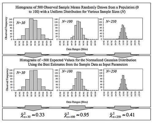
Remember central limit theorem!
Not significant –> retain null hypothesis, not significantly different from normal distribution.
data_eur<-filter(data_no_miss, GRP=='0')
data_asian_i<-filter(data_no_miss, GRP=='1')
data_asian_a<-filter(data_no_miss, GRP=='2')
# You would do this for all 3!
shapiro.test(data_asian_a$O)
##
##  Shapiro-Wilk normality test
##
## data:  data_asian_a$O
## W = 0.96901, p-value = 0.1584
Beware K-S test: easily significant!
ks.test(data_asian_a$O, "pnorm") #pnorm --> normal distribution
##
##  One-sample Kolmogorov-Smirnov test
##
## data:  data_asian_a$O
## D = 1, p-value < 2.2e-16
## alternative hypothesis: two-sided
Recommendation check normality visually! (histogram / violin plot / …)
Think back to the 'Datasaurus'.

??nortest package. Read the vignette and references.
Anderson-Darling test.
Cramer-von Mises test.
Lilliefors test (K-S) (correction of K-S).
Shapiro-Francia test.
Jarque Bera test (+ adjusted).
Bartlett's test - assumes normality.
If significant could also point to deviation in normality as opposed to violation of the assumption of homogeneity of variance.
bartlett.test(O ~ GRP, data=data_no_miss)
##
##  Bartlett test of homogeneity of variances
##
## data:  O by GRP
## Bartlett's K-squared = 3.1821, df = 2, p-value = 0.2037
Levene's test does not assume normality.
require(car) # package which does test
require(dplyr)
# need to make it a factor!
data_no_miss$GRP_fact<-as_factor(data_no_miss$GRP)
leveneTest(O ~ GRP_fact, data=data_no_miss)
## Levene's Test for Homogeneity of Variance (center = median)
##        Df F value Pr(>F)
## group   2  1.7076 0.1839
##       200
Assumptions upheld here!
Sample write up: Visual inspection suggested that the distribution of the dependent variable is close to normal. A Levene's test suggests that the assumption of homogeneity of variances is not violated, F(2,200) = 1.71, p= .18)
We can move on to ANOVA!

As an aside: you could mention, the platykurtosis in the Asian American group.
(In your assignment I would count both correct in this case).


Test the assumptions for an ANOVA with Extraversion (E) and group as independent variable.

Why this matters will become clearer when we discuss.
Analysis of variance.
Anova1<-aov(O ~ GRP_fact, data=data_no_miss)
summary(Anova1)
##              Df Sum Sq Mean Sq F value   Pr(>F)
## GRP_fact      2   8774    4387   15.05 8.13e-07 ***
## Residuals   200  58284     291
## ---
## Signif. codes:  0 '***' 0.001 '**' 0.01 '*' 0.05 '.' 0.1 ' ' 1
Anova2<-lm(O~ GRP_fact, data=data_no_miss)
summary(Anova2)
##
## Call:
## lm(formula = O ~ GRP_fact, data = data_no_miss)
##
## Residuals:
##     Min      1Q  Median      3Q     Max
## -41.400 -11.982  -0.982  11.828  41.600
##
## Coefficients:
##                              Estimate Std. Error t value Pr(>|t|)
## (Intercept)                   113.400      1.971  57.529  < 2e-16 ***
## GRP_factAsian Internationals   -2.039      2.817  -0.724     0.47
## GRP_factAsian Americans        13.582      3.015   4.505 1.13e-05 ***
## ---
## Signif. codes:  0 '***' 0.001 '**' 0.01 '*' 0.05 '.' 0.1 ' ' 1
##
## Residual standard error: 17.07 on 200 degrees of freedom
## Multiple R-squared:  0.1308, Adjusted R-squared:  0.1222
## F-statistic: 15.05 on 2 and 200 DF,  p-value: 8.126e-07
summary prints parameter tests but should you be after the F-test.
anova(Anova2)
## Analysis of Variance Table
##
## Response: O
##            Df Sum Sq Mean Sq F value    Pr(>F)
## GRP_fact    2   8774  4387.0  15.054 8.126e-07 ***
## Residuals 200  58284   291.4
## ---
## Signif. codes:  0 '***' 0.001 '**' 0.01 '*' 0.05 '.' 0.1 ' ' 1
For your reference. drop1 can also get you some relevant key info.
Don't worry about AIC for now. It is a model fit statistic (lower = better). More about this when we discuss multilevel models.
drop1(Anova2) # some additional info. ??drop1
## Single term deletions
##
## Model:
## O ~ GRP_fact
##          Df Sum of Sq   RSS    AIC
## <none>                58284 1155.0
## GRP_fact  2      8774 67058 1179.4
Best bet for replicating SPSS results!
require(ez)
Ez_ANOVA1<-ezANOVA(data_no_miss, dv=O, wid=ID, between=GRP_fact, detailed=TRUE)
Ez_ANOVA1
## $ANOVA
##     Effect DFn DFd      SSn      SSd        F            p p<.05       ges
## 1 GRP_fact   2 200 8773.973 58283.59 15.05393 8.125554e-07     * 0.1308424
##
## $`Levene's Test for Homogeneity of Variance`
##   DFn DFd      SSn      SSd        F       p p<.05
## 1   2 200 356.9336 20903.13 1.707561 0.18394
Effect size measure!
ges= Generalized Eta-Squared. \(\eta^2_g\) . There is also partial \(\eta^2\). Read more here.
How to do Greek symbols and mathematical functions? here or check the .rmd for this lecture.
If you are up for a challenge. You can figure out how to calculate this effect size measure on your own!.

A one-way ANOVA showed a significant effect of cultural group on openness to experience F(2, 200) = 15.05, p < .0001, \(\eta^2_g\) = .13.
require(apaTables)
apa.aov.table(Anova1, filename="APA_Anova_Table.doc", table.number = 1)
##
##
## Table 1
##
## ANOVA results using O as the dependent variable
##
##
##    Predictor        SS  df        MS       F    p partial_eta2
##  (Intercept) 964467.00   1 964467.00 3309.57 .000
##     GRP_fact   8773.97   2   4386.98   15.05 .000          .13
##        Error  58283.59 200    291.42
##  CI_90_partial_eta2
##
##          [.06, .20]
##
##
## Note: Values in square brackets indicate the bounds of the 90% confidence interval for partial eta-squared
Where does the difference lie?

resultTukey<-TukeyHSD(Anova1)
resultTukey
##   Tukey multiple comparisons of means
##     95% family-wise confidence level
##
## Fit: aov(formula = O ~ GRP_fact, data = data_no_miss)
##
## $GRP_fact
##                                              diff       lwr       upr
## Asian Internationals-European Americans -2.038889 -8.689634  4.611856
## Asian Americans-European Americans      13.582143  6.463135 20.701151
## Asian Americans-Asian Internationals    15.621032  8.438902 22.803161
##                                             p adj
## Asian Internationals-European Americans 0.7496332
## Asian Americans-European Americans      0.0000335
## Asian Americans-Asian Internationals    0.0000020
Have you heard of post-hoc corrections? Why do they exist?
Read more here and use them sensibly.
Why Bonferroni should be abandoned (in medicine and ecology).

You can make a prettier layout. By changing the variable names, etc. You can also change the labels it prints.
Totally check out stargazer!
require(broom)
require(stargazer)
# Broom turns our result into a dataframe!
# We can then 'tidy' it and make a report!
tidy_resultTukey<-tidy(resultTukey)
stargazer(tidy_resultTukey, summary = F, type="html", out="Tukey.html")
Alternative. This will also have Cohen's d effect size values.
require(apaTables)
apa.d.table(iv=GRP_fact, dv=O, data=data_no_miss, filename="Table_1_APA_tukey.doc", show.conf.interval=T, landscape=T, table.number = 1)
##
##
## Table 1
##
## Means, standard deviations, and d-values with confidence intervals
##
##
##   Variable                M      SD    1             2
##   1. European Americans   113.40 17.12
##
##   2. Asian Internationals 111.36 15.24 0.13
##                                        [-0.20, 0.45]
##
##   3. Asian Americans      126.98 19.11 0.75          0.92
##                                        [0.40, 1.11]  [0.55, 1.28]
##
##
## Note. M and SD are used to represent mean and standard deviation, respectively.
## Values in square brackets indicate the 95% confidence interval for each d-value.
## The confidence interval is a plausible range of population d-values
## that could have caused the sample d-value (Cumming, 2014).
## d-values are estimates calculated using formulas 4.18 and 4.19
## from Borenstein, Hedges, Higgins, & Rothstein (2009).
## d-values not calculated if unequal variances prevented pooling.
##
How would you have proceeded, if the assumptions were violated?

They do not assume a normal distribution but can be less powerful.
Many options exist. You can read and find others (see references).

The t1way function computes a one-way ANOVA for the trimmed means. Homoscedasticity assumption not required.
lincoln() for the posthoc tests.
#WRS.
require(WRS2)
t1way(O ~ GRP_fact, data=data_no_miss)
## Call:
## t1way(formula = O ~ GRP_fact, data = data_no_miss)
##
## Test statistic: F = 11.067
## Degrees of freedom 1: 2
## Degrees of freedom 2: 74.67
## p-value: 6e-05
##
## Explanatory measure of effect size: 0.44
The t1waybt function computes a one-way ANOVA for the trimmed means.
# Specify Between.
t1waybt(O ~ GRP_fact, data=data_no_miss, nboot=10000)
## Call:
## t1waybt(formula = O ~ GRP_fact, data = data_no_miss, nboot = 10000)
##
## Effective number of bootstrap samples was 10000.
##
## Test statistic: 11.067
## p-value: 1e-04
## Variance explained 0.192
## Effect size 0.439
Computes a one-way ANOVA for the medians. Homoscedasticity assumption not required. Avoid too many ties.
# WRS, ANOVA for Medians. (note iter=)
med1way(O ~ GRP_fact, data=data_no_miss, iter=10000)
## Call:
## med1way(formula = O ~ GRP_fact, data = data_no_miss, iter = 10000)
##
## Test statistic F: 6.6673
## Critical value: 3.2621
## p-value: 0.0036
# analysis of Medians leads to same conclusion.
Read through WRS2 manual or Wilcox (2012) to find out more.
Permutation tests use random shuffles of the data to get the correct distribution of a test statistic under a null hypothesis. (No power issue by the way)
Shuffles are not the same as bootstraps. Some assumptions do still apply (e.g., non-independence of observations).
require(coin)
independence_test(O ~ GRP_fact, data=data_no_miss)
##
##  Asymptotic General Independence Test
##
## data:  O by
##   GRP_fact (European Americans, Asian Internationals, Asian Americans)
## maxT = 5.0961, p-value = 8.742e-07
## alternative hypothesis: two.sided
A permutation test via the 'coin' package showed that there are significant differences between the three groups in Openness to Experience (maxT= 5.10, p< .0001).
(Note post-hoc tests are currently unavailable via 'coin' but you can get them via 'rcompanion', more here)
The difference is the C. Covariate.
Often we want to control for a potential confound, so suppose that you are testing a new weight loss drug. You could analyse the participant's weight at the end of the trial while partialling out their start weight. This would be an ANCOVA scenario (but beware).
Beware of Lord's paradox. If one researcher calculates a change score and runs an independent samples t-test while the other runs an ANCOVA
The order in which you put in things matters!!
# Type I errors
lm_ancova<-lm(O~E+GRP_fact, data=data_no_miss)
anova(lm_ancova)
## Analysis of Variance Table
##
## Response: O
##            Df Sum Sq Mean Sq F value    Pr(>F)
## E           1   8349  8348.9  34.339 1.894e-08 ***
## GRP_fact    2  10325  5162.7  21.234 4.379e-09 ***
## Residuals 199  48383   243.1
## ---
## Signif. codes:  0 '***' 0.001 '**' 0.01 '*' 0.05 '.' 0.1 ' ' 1
# note that the order matters for the F-tests.
lm_ancova2<-lm(O~GRP_fact+E, data=data_no_miss)
anova(lm_ancova2)
## Analysis of Variance Table
##
## Response: O
##            Df Sum Sq Mean Sq F value    Pr(>F)
## GRP_fact    2   8774  4387.0  18.044 6.289e-08 ***
## E           1   9900  9900.3  40.720 1.209e-09 ***
## Residuals 199  48383   243.1
## ---
## Signif. codes:  0 '***' 0.001 '**' 0.01 '*' 0.05 '.' 0.1 ' ' 1
Type I,II,III errors.
For now, you should be aware that type of errors matters (I,II,III). read more here and here
SPSS uses type III. So let's aim to emulate (even though that might not always be optimal)
# Type III errors
require(car)
require(compute.es)
Ancova<-lm(O~GRP_fact+E, contrasts=list(GRP_fact=contr.sum), data=data_no_miss)
Anova(Ancova, type="III")
## Anova Table (Type III tests)
##
## Response: O
##             Sum Sq  Df F value    Pr(>F)
## (Intercept)  25976   1 106.838 < 2.2e-16 ***
## GRP_fact     10325   2  21.234 4.379e-09 ***
## E             9900   1  40.720 1.209e-09 ***
## Residuals    48383 199
## ---
## Signif. codes:  0 '***' 0.001 '**' 0.01 '*' 0.05 '.' 0.1 ' ' 1
require(multcomp)
posth=glht(Ancova, linfct=mcp(GRP_fact="Tukey"))
summary(posth) ##shows the output in a nice format
##
##   Simultaneous Tests for General Linear Hypotheses
##
## Multiple Comparisons of Means: Tukey Contrasts
##
##
## Fit: lm(formula = O ~ GRP_fact + E, data = data_no_miss, contrasts = list(GRP_fact = contr.sum))
##
## Linear Hypotheses:
##                                                Estimate Std. Error t value
## Asian Internationals - European Americans == 0    4.837      2.789   1.734
## Asian Americans - European Americans == 0        17.870      2.835   6.304
## Asian Americans - Asian Internationals == 0      13.033      2.808   4.642
##                                                Pr(>|t|)
## Asian Internationals - European Americans == 0    0.195
## Asian Americans - European Americans == 0        <1e-04 ***
## Asian Americans - Asian Internationals == 0      <1e-04 ***
## ---
## Signif. codes:  0 '***' 0.001 '**' 0.01 '*' 0.05 '.' 0.1 ' ' 1
## (Adjusted p values reported -- single-step method)
A one-way ANCOVA was conducted to compare Openness across groups whilst controlling for Extraversion. There was a significant effect of cultural group, F(2,199)=21.23, p<.0001. In addition, the effect of the covariate, Extraversion, was significant, F(1,199)=40.72, p<.0001.
You would then describe the post-hoc differences and also explore how extraversion is associated with (e.g., correlation, plot.)
Look at the 'lmPerm' package and this.
All the previous assumptions + (+ multicollinearity (not an assumption but a problem)
Multivariate normality
Homogeneity of co-variances.
Multivariate Shapiro test. (The Univariate's test bigger brother…).
Sensitive to sample size, if large small deviations will lead to significance.
require(RVAideMemoire)
multivariatenorm<-dplyr::select(data_no_miss, -GRP_fact, -GRP,-ID)
mshapiro.test(multivariatenorm)
##
##  Multivariate Shapiro-Wilk normality test
##
## data:  (N,E,O,A,C)
## W = 0.98577, p-value = 0.03887
A whole host of alternatives. More here.
require(MVN) # Alternative method, one example
mvn(multivariatenorm)
## $multivariateNormality
##              Test        Statistic            p value Result
## 1 Mardia Skewness 57.0115702615851 0.0107887129793524     NO
## 2 Mardia Kurtosis  1.9394290567207 0.0524491152485054    YES
## 3             MVN             <NA>               <NA>     NO
##
## $univariateNormality
##           Test  Variable Statistic   p value Normality
## 1 Shapiro-Wilk     N        0.9942    0.6210    YES
## 2 Shapiro-Wilk     E        0.9897    0.1552    YES
## 3 Shapiro-Wilk     O        0.9893    0.1360    YES
## 4 Shapiro-Wilk     A        0.9915    0.2815    YES
## 5 Shapiro-Wilk     C        0.9889    0.1158    YES
##
## $Descriptives
##     n     Mean  Std.Dev Median Min Max  25th  75th       Skew   Kurtosis
## N 203  95.9064 21.23737     97  36 160  81.0 109.5 -0.1442702 -0.1102764
## E 203 116.7291 19.93406    117  50 175 103.0 129.5 -0.1039661  0.6504353
## O 203 116.4236 18.21999    115  72 166 104.0 127.0  0.3079877 -0.1699643
## A 203 113.9261 18.29136    115  58 161 103.0 127.0 -0.2962256  0.1136037
## C 203 111.7734 18.53971    112  57 171  98.5 124.0  0.1476949  0.4428221
Violated (but could be way worse, trust me … )
mvn(multivariatenorm, multivariatePlot = "qq")

## $multivariateNormality
##              Test        Statistic            p value Result
## 1 Mardia Skewness 57.0115702615851 0.0107887129793524     NO
## 2 Mardia Kurtosis  1.9394290567207 0.0524491152485054    YES
## 3             MVN             <NA>               <NA>     NO
##
## $univariateNormality
##           Test  Variable Statistic   p value Normality
## 1 Shapiro-Wilk     N        0.9942    0.6210    YES
## 2 Shapiro-Wilk     E        0.9897    0.1552    YES
## 3 Shapiro-Wilk     O        0.9893    0.1360    YES
## 4 Shapiro-Wilk     A        0.9915    0.2815    YES
## 5 Shapiro-Wilk     C        0.9889    0.1158    YES
##
## $Descriptives
##     n     Mean  Std.Dev Median Min Max  25th  75th       Skew   Kurtosis
## N 203  95.9064 21.23737     97  36 160  81.0 109.5 -0.1442702 -0.1102764
## E 203 116.7291 19.93406    117  50 175 103.0 129.5 -0.1039661  0.6504353
## O 203 116.4236 18.21999    115  72 166 104.0 127.0  0.3079877 -0.1699643
## A 203 113.9261 18.29136    115  58 161 103.0 127.0 -0.2962256  0.1136037
## C 203 111.7734 18.53971    112  57 171  98.5 124.0  0.1476949  0.4428221
Solution: Check for outliers, run analyses again. Report both!
Transformations. Box-Cox transform.
Central limit theorem to the rescue again! (also note Hotelling's T^2 robust)

As with the univariate case. So, you would run a series of tests such as Levene's Test and examine those.
Not done here but you can run these on your own.
Approach with care.
Very easily significant. Therefore, usually p=.001 as threshold. More here.
require(heplots) #alternative is 'biotools' package.
boxM(multivariatenorm, data_no_miss$GRP)
##
##  Box's M-test for Homogeneity of Covariance Matrices
##
## data:  multivariatenorm
## Chi-Sq (approx.) = 40.668, df = 30, p-value = 0.09256
Manovamodel <- manova(cbind(N,E,A,O,C) ~ GRP_fact, data = data_no_miss)
summary(Manovamodel)
##            Df  Pillai approx F num Df den Df    Pr(>F)
## GRP_fact    2 0.41862    10.43     10    394 1.106e-15 ***
## Residuals 200
## ---
## Signif. codes:  0 '***' 0.001 '**' 0.01 '*' 0.05 '.' 0.1 ' ' 1
Other measures exist but Pillai's Trace is typically most common. You can find out more about them here. Also about the math (also see references).

Pillai's Trace most commonly reported.
Sample report: A MANOVA was conducted with five dependent variables (Neuroticism, Extraversion, Conscientousness, Agreeableness, and Openness to Experience) and cultural group as the between-subject factor. A statistically significant effect was found (Pillai's Trace= .42, F(10,394)=10.43, p<.0001).
You would then report follow-up tests! (e.g., Univariate ANOVA's)
In conclusion the personality profiles differ between these 3 groups.
Univariate ANOVA's / plot your data / Discriminant analysis.
Using last week's Salaries dataset, test the assumptions for an ANOVA with monthly salary as dependent variable and academic rank as independent variable.
Conduct an ANOVA with the appropriate post-hoc tests. What do you conclude?
Conduct an alternative non-parametric test to the ANOVA. What do you conclude.
Conduct an ANCOVA with gender as factor, and years since Ph.D. as covariate. What do you conclude?
Load the iris dataset, it is part of the datasets package.
It is a famous dataset with measurements of 3 species of iris flowers.
Test the assumptions for a MANOVA with Species as the between-subject factor and petal length and sepal length as dependent variables.
Run the MANOVA. What do you conclude? Write up the result as you would do for a paper?
BONUS: Plot one of the results from your analyses on the salaries database.
BONUS: Conduct a follow up analysis or plot for the MANOVA.