- Last week: Correlation, OLS Regression, Logistic regression
- Today: Moderation effects. 2 x 2 ANOVA
2018-10-26 | disclaimer
PY0782: Advanced Quantitative research methods.
Goals (today)
ANOVA (again… .)
Assumptions underpinning ANOVA
two-way ANOVA + plot.
Assignment
After today you should be able to complete the following sections:
Two-way ANOVA
Plots (you could already do this!)
After today.
You can complete the entire assignment I !! Easy marks to gain, if you can’t figure something out, move on to the next bit. Three different datasets, so you can really chunk it.
Work through the exercises first, if you have not done so! It will give you insight in how to tackle the assignment.
Questions in discussion board on Blackboard.

Types of errors (I,II,III).
Before we move on:
Initially ANOVA was designed for balanced designs: equal N for each factor.
When unbalanced: different ways for calculating Sums of Squares.

Type of errors
If everything is uncorrelated as in A below then it does not matter at all. However, if the predictors correlate then there are several options. More info here and here.

Terminology
Type I SS (“sequential”): Order-dependent. (Assuming we put A first in the order, then SS[A] = t + u + v + w; SS[B] = x + y; SS[A*B] = z)
Type II SS (“hierarchical”): SS[A] = t + w; SS[B] = x + y; SS[A*B] = z. Adjusts terms for all other terms except higher-order terms including the same predictors.
Type III SS (“marginal”, “orthogonal”): SS[A] = t; SS[B] = x; SS[A*B] = z. This assesses the contribution of each predictor over and above all others.
Which one to use?
Pick the type corresponding to your hypothesis! If you have strong theoretical predictions for A and want to control for things then perhaps type I is your choice. (But most of the time the choice is between II and III.).
For the highest order interaction all will give the same answer.
Type II: most powerful when no interaction present. (note different interpretation of main effects when interaction is present.)
Type III: conservative (with regards to main effects).
Interaction effects?
Can anybody explain what an interaction effect is?
What is an example? And why should we particularly care in psychology?
Synonyms
Moderation = Interaction.
Moderation is not the same as mediation. (More about that soon.)
Multiplying of terms.

Two-way ANOVA (2x2 or 2x3 for example)
Check the relevant assumptions first.
Do you recall what these are? (look back to slides from week 3 if you do not remember)
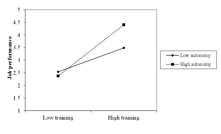
Graphical example.
Often you see these types of plots… .
Talk to your neighbour.
Have you come across an interaction design in your internship or Ba.-Thesis.
What shape was it?

Other forms?
What other forms can interactions take?
Two-way / Three-way.

ToothGrowth dataset.
From datasets package. (ToothGrowth).
From vignette: The response is the length of odontoblasts (cells responsible for tooth growth) in 60 guinea pigs. Each animal received one of three dose levels of vitamin C (0.5, 1, and 2 mg/day) by one of two delivery methods, (orange juice or ascorbic acid (a form of vitamin C and coded as VC).
Assumption checks.
Load the data (ToothGrowth) and test the assumptions for a 2 x 3 ANOVA. Go back to your notes from lecture 3 if you need to. (hint: visual checks / homogeneity of variance). You’ll need to convert dose to a factor (as.factor)
What are the solutions, in case of violations?
Check your solution here

Notations. (Crawley, 2013:396)
Expressions :
+ indicates inclusion of an explanatory variable in the model (not addition);
- indicates deletion of an explanatory variable from the model (not subtraction);
* indicates inclusion of explanatory variables and interactions (not multiplication);
/ indicates nesting of explanatory variables in the model (not division);
| indicates conditioning (not ‘or’), so that y~x | z is read as ‘y as a function of x given z’.
More Notations.
Factorial ANOVA: y~N*P*K
N, P and K are two-level factors to be fitted along with all their interactions
Three-way ANOVA: y~N*P*K - N:P:K
As above, but do not fit the three-way interaction, fit all two-way interactions.
Interactions require lower order effects.
If you are testing a higher order interaction, you need all the lower level effects.
So when testing a three-way interaction, you would include all two-way interactions and all main defects.
Interaction Anova.
setwd("~/Dropbox/Teaching_MRes_Northumbria/Lecture5")
require(car)
## Loading required package: car
## Loading required package: carData
ToothGrowth2<-ToothGrowth
ToothGrowth2$dose<-as.factor(ToothGrowth$dose)
# This ensures you get the same results as beloved SPSS.
options(contrasts = c("contr.helmert", "contr.poly")) # change options.
 # need this for correct SS. - type command
ANOVAtwobythree<-Anova(lm(len~supp*dose, data=ToothGrowth2), type = 3)
Results.
ANOVAtwobythree
## Anova Table (Type III tests)
##
## Response: len
##              Sum Sq Df  F value    Pr(>F)
## (Intercept) 21236.5  1 1610.393 < 2.2e-16 ***
## supp          205.4  1   15.572 0.0002312 ***
## dose         2426.4  2   92.000 < 2.2e-16 ***
## supp:dose     108.3  2    4.107 0.0218603 *
## Residuals     712.1 54
## ---
## Signif. codes:  0 '***' 0.001 '**' 0.01 '*' 0.05 '.' 0.1 ' ' 1
Alternative route.
# alternative route. Notice that the options are different here!
options(contrasts = c("contr.sum","contr.poly"))
ANOVAtwobythree_alt<-lm(len~supp*dose, data=ToothGrowth2)
summary(ANOVAtwobythree_alt)
##
## Call:
## lm(formula = len ~ supp * dose, data = ToothGrowth2)
##
## Residuals:
##    Min     1Q Median     3Q    Max
##  -8.20  -2.72  -0.27   2.65   8.27
##
## Coefficients:
##             Estimate Std. Error t value Pr(>|t|)
## (Intercept)  18.8133     0.4688  40.130  < 2e-16 ***
## supp1         1.8500     0.4688   3.946 0.000231 ***
## dose1        -8.2083     0.6630 -12.381  < 2e-16 ***
## dose2         0.9217     0.6630   1.390 0.170190
## supp1:dose1   0.7750     0.6630   1.169 0.247568
## supp1:dose2   1.1150     0.6630   1.682 0.098394 .
## ---
## Signif. codes:  0 '***' 0.001 '**' 0.01 '*' 0.05 '.' 0.1 ' ' 1
##
## Residual standard error: 3.631 on 54 degrees of freedom
## Multiple R-squared:  0.7937, Adjusted R-squared:  0.7746
## F-statistic: 41.56 on 5 and 54 DF,  p-value: < 2.2e-16
Alternative route: F-test
drop1(ANOVAtwobythree_alt, .~., test="F")
## Single term deletions
##
## Model:
## len ~ supp * dose
##           Df Sum of Sq     RSS    AIC F value    Pr(>F)
## <none>                  712.11 160.43
## supp       1    205.35  917.46 173.64  15.572 0.0002312 ***
## dose       2   2426.43 3138.54 245.43  92.000 < 2.2e-16 ***
## supp:dose  2    108.32  820.43 164.93   4.107 0.0218603 *
## ---
## Signif. codes:  0 '***' 0.001 '**' 0.01 '*' 0.05 '.' 0.1 ' ' 1
Ez.
return_aov will return an ANOVA list from which we can then call objects
# make an ID variable
ToothGrowth2$id <- seq(1:60)
require(ez)
ez <- ezANOVA(data = ToothGrowth2, dv = .(len), wid = .(id),
    between = .(supp, dose), return_aov = T, detailed = TRUE,
    type = 3)
Ez output
ez
## $ANOVA
##        Effect DFn DFd       SSn     SSd           F            p p<.05
## 1 (Intercept)   1  54 21236.491 712.106 1610.392970 6.939976e-42     *
## 2        supp   1  54   205.350 712.106   15.571979 2.311828e-04     *
## 3        dose   2  54  2426.434 712.106   91.999965 4.046291e-18     *
## 4   supp:dose   2  54   108.319 712.106    4.106991 2.186027e-02     *
##         ges
## 1 0.9675557
## 2 0.2238254
## 3 0.7731092
## 4 0.1320279
##
## $`Levene's Test for Homogeneity of Variance`
##   DFn DFd    SSn     SSd        F         p p<.05
## 1   5  54 38.926 246.053 1.708578 0.1483606
##
## $aov
## Call:
##    aov(formula = formula(aov_formula), data = data)
##
## Terms:
##                     supp     dose supp:dose Residuals
## Sum of Squares   205.350 2426.434   108.319   712.106
## Deg. of Freedom        1        2         2        54
##
## Residual standard error: 3.631411
## Estimated effects may be unbalanced
Export.
If you want exports you’ll need the ‘car’ or ‘ez’ objects route.
If you want to make it prettier, you would change the labels in the dataframe (and consider dropping certain columns (e.g., the star notation)).
require(stargazer)
stargazer(ANOVAtwobythree, summary = F, type="html", out="ANOVA_2_3.html")
stargazer(ez$ANOVA, summary = F, type="html", out="ez_2_3.html")
Sample write up.
A two-way ANOVA was conducted to examine the effect of supplement and dose on growth of odontoblasts. There was a significant interaction effect between supplement and dose, F(2,54)= 4.11, p= .022, \(\eta^2_g\)= .13.
You would then further explore the contrasts or plot the results.
Post-hoc tests.
TukeyHSD(ez$aov, which="dose")
##   Tukey multiple comparisons of means
##     95% family-wise confidence level
##
## Fit: aov(formula = formula(aov_formula), data = data)
##
## $dose
##         diff       lwr       upr   p adj
## 1-0.5  9.130  6.362488 11.897512 0.0e+00
## 2-0.5 15.495 12.727488 18.262512 0.0e+00
## 2-1    6.365  3.597488  9.132512 2.7e-06
alternative
library(multcomp)
summary(glht(ez$aov, linfct = mcp(dose = "Tukey")))
##
##   Simultaneous Tests for General Linear Hypotheses
##
## Multiple Comparisons of Means: Tukey Contrasts
##
##
## Fit: aov(formula = formula(aov_formula), data = data)
##
## Linear Hypotheses:
##              Estimate Std. Error t value Pr(>|t|)
## 1 - 0.5 == 0    9.130      1.148   7.951   <1e-05 ***
## 2 - 0.5 == 0   15.495      1.148  13.493   <1e-05 ***
## 2 - 1 == 0      6.365      1.148   5.543   <1e-05 ***
## ---
## Signif. codes:  0 '***' 0.001 '**' 0.01 '*' 0.05 '.' 0.1 ' ' 1
## (Adjusted p values reported -- single-step method)
Plot to show the interaction?
ggpubr makes ggplot2 even easier, and churns out some beautiful graphs.
require(ggpubr)
plot_moderation <- ggviolin(ToothGrowth2, x = "dose",
    y = "len", color = "dose", palette = c("black",
        "darkblue", "darkred"), add = c("jitter", "boxplot"),
    shape = "dose") + labs(x = "Condition", y = "Length",
    color = "Dose", shape = "Dose")
plot_moderation + facet_wrap(~supp)

# Jitter could be omitted
Export Means and SD.
require(apaTables)
apa.2way.table(supp, dose, len, ToothGrowth2, filename = "toothgrowth ANOVA",
    table.number = 1, show.conf.interval = T, show.marginal.means = T,
    landscape = TRUE)
##
##
## Table 1
##
## Means and standard deviations for len as a function of a 2(supp) X 3(dose) design
##
##               M       M_95%_CI   SD
##  dose:0.5
##      supp
##        OJ 13.23 [10.04, 16.42] 4.46
##        VC  7.98   [6.02, 9.94] 2.75
##
##    dose:1
##      supp
##        OJ 22.70 [19.90, 25.50] 3.91
##        VC 16.77 [14.97, 18.57] 2.52
##
##    dose:2
##      supp
##        OJ 26.06 [24.16, 27.96] 2.66
##        VC 26.14 [22.71, 29.57] 4.80
##
## Note. M and SD represent mean and standard deviation, respectively.
## LL and UL indicate the lower and upper limits of the
## 95% confidence interval for the mean, respectively.
## The confidence interval is a plausible range of population means
## that could have created a sample mean (Cumming, 2014).
Bootstrap!
Note the singular.ok = T statement.
# Bootstrap CI for ANOVA
library(boot)
# function to obtain p.values from F-test from the
# data
p_value_twowayaov <- function(data, indices) {
    data_boot <- data[indices, ]  # allows boot to select sample
    ANOVAtwobytwo_boot <- Anova(lm(len ~ supp * dose,
        data = data_boot), contrasts = c("contr.sum",
        "contr.poly"), type = 3, singular.ok = TRUE)
    return(ANOVAtwobytwo_boot$`Pr(>F)`[4])
}
# bootstrapping with 1000 replications
set.seed(1234)
results_twowayaov <- boot(data = ToothGrowth2, statistic = p_value_twowayaov,
    R = 1000)
Bootstrap results
# view results
results_twowayaov
##
## ORDINARY NONPARAMETRIC BOOTSTRAP
##
##
## Call:
## boot(data = ToothGrowth2, statistic = p_value_twowayaov, R = 1000)
##
##
## Bootstrap Statistics :
##       original     bias    std. error
## t1* 0.02186027 0.04918218   0.1434026
Bootstrap plots
89% CI - check here why.
plot(results_twowayaov)

CI
# get 89% confidence interval
boot.ci(results_twowayaov, conf = 0.89, type="bca")
## BOOTSTRAP CONFIDENCE INTERVAL CALCULATIONS
## Based on 1000 bootstrap replicates
##
## CALL :
## boot.ci(boot.out = results_twowayaov, conf = 0.89, type = "bca")
##
## Intervals :
## Level       BCa
## 89%   ( 0.0002,  0.6498 )
## Calculations and Intervals on Original Scale
tree
Three are ways to “automate” this search for interaction, and there are ‘tree’ based models which will uncover interactions.
require(tree)
tree <- tree(len ~ ., ToothGrowth)
plot(tree)
text(tree)

‘party’!
Read about ??party. Amazing package to find patterns in your data. (It does so in a very clever way. )
require(party)
ctree <- ctree(len ~ ., ToothGrowth)
Party= Recursive Partitioning of Variance. (underpinning it is permutation testing…)

plot
plot(ctree)

Continuous variables and interactions
Back to the Salaries dataset.
require(car)
salaries<-carData::Salaries
require(dplyr)
salaries<- salaries %>% mutate(monthly_salary=salary/9)
salaries<- salaries %>% mutate(yrs.since.phd_cent= yrs.since.phd -mean(yrs.since.phd))
names(salaries)[5] <- "gender" # renamed
Interaction between continuous and dichotomous.
Regression model.
interaction<-lm(monthly_salary~gender*yrs.since.phd_cent,data=salaries)
summary(interaction)
##
## Call:
## lm(formula = monthly_salary ~ gender * yrs.since.phd_cent, data = salaries)
##
## Residuals:
##    Min     1Q Median     3Q    Max
##  -9224  -2160   -332   1673  11406
##
## Coefficients:
##                            Estimate Std. Error t value Pr(>|t|)
## (Intercept)                12503.16     295.75  42.276  < 2e-16 ***
## gender1                     -220.27     295.75  -0.745    0.457
## yrs.since.phd_cent           142.32      26.00   5.473 7.88e-08 ***
## gender1:yrs.since.phd_cent    40.44      26.00   1.555    0.121
## ---
## Signif. codes:  0 '***' 0.001 '**' 0.01 '*' 0.05 '.' 0.1 ' ' 1
##
## Residual standard error: 3047 on 393 degrees of freedom
## Multiple R-squared:  0.1867, Adjusted R-squared:  0.1805
## F-statistic: 30.07 on 3 and 393 DF,  p-value: < 2.2e-16
Post-hoc interactions.
phia package (can do quick basic plots)
require(phia)
means_int <- interactionMeans(interaction)
plot(means_int)

Test interactions (phia)
Not useful here as only 2 levels, but for model with 3 this is how you would get the post-hoc tests.
testInteractions(interaction)
## F Test:
## P-value adjustment method: holm
##               Value  Df  Sum of Sq      F Pr(>F)
## Female-Male -440.53   1    5148409 0.5547 0.4569
## Residuals           393 3647788770
Basic plot.
You can modify this. Alternatively look to ggplot2 (Basically a scatterplot with grouping).
library(effects)
plot(allEffects(interaction), multiline=TRUE, ci.style="bands")

Try it yourself
Conduct a 2 x 2 ANOVA with gender (or sex if you don’t want to rename…) and yrs.service (center it first).
Make a plot.

Permutation tests.
We can again do something clever, permutations! More here and the ‘vegan’ manual.
library(vegan)
ToothGrowth2<-ToothGrowth
attach(ToothGrowth2) # need to attach data
# margin corresponds to type III error.
adonis2(len~ supp*dose, data = ToothGrowth2, by='margin', method='euclidean')
## Permutation test for adonis under reduced model
## Marginal effects of terms
## Permutation: free
## Number of permutations: 999
##
## adonis2(formula = len ~ supp * dose, data = ToothGrowth2, method = "euclidean", by = "margin")
##           Df SumOfSqs      R2      F Pr(>F)
## supp:dose  1     88.9 0.02576 5.3335  0.022 *
## Residual  56    933.6 0.27045
## Total     59   3452.2 1.00000
## ---
## Signif. codes:  0 '***' 0.001 '**' 0.01 '*' 0.05 '.' 0.1 ' ' 1
continuous x continuous interaction
The following example data (epi.bfi) comes from the psych package (Revelle, 2012), 231 undergraduate students.
bdi = Beck Depression Inventory
epiNeur = Neuroticism from Eysenck Personality Inventory
stateanx = state anxiety
Does the relation between neuroticism (X) and depression (Y) depend on state-anxiety (Z)? (Basic example - consider centering when you run it yourself - easier to interpret reduces multicollinearity issues).
Model
require(psych)
interaction2<-lm(bdi ~ stateanx*epiNeur, data=epi.bfi)
summary(interaction2)
##
## Call:
## lm(formula = bdi ~ stateanx * epiNeur, data = epi.bfi)
##
## Residuals:
##      Min       1Q   Median       3Q      Max
## -12.0493  -2.2513  -0.4707   2.1135  11.9949
##
## Coefficients:
##                  Estimate Std. Error t value Pr(>|t|)
## (Intercept)       0.06367    2.18559   0.029   0.9768
## stateanx          0.03750    0.06062   0.619   0.5368
## epiNeur          -0.14765    0.18869  -0.782   0.4347
## stateanx:epiNeur  0.01528    0.00466   3.279   0.0012 **
## ---
## Signif. codes:  0 '***' 0.001 '**' 0.01 '*' 0.05 '.' 0.1 ' ' 1
##
## Residual standard error: 4.12 on 227 degrees of freedom
## Multiple R-squared:  0.4978, Adjusted R-squared:  0.4912
## F-statistic: 75.02 on 3 and 227 DF,  p-value: < 2.2e-16
Plot.
Usually we are interested in shifts of one SD.
library(rockchalk)
plotCurves(interaction2, plotx = "epiNeur", modx = "stateanx",
    modxVals = "std.dev.", interval = "confidence")

Simple slopes method.
require(jtools)
sim_slopes(interaction2, pred = epiNeur, modx = stateanx,
    johnson_neyman = FALSE)
## SIMPLE SLOPES ANALYSIS
##
## Slope of epiNeur when stateanx = 51.33 (+ 1 SD):
##  Est. S.E. t val.    p
##  0.64 0.09   7.20 0.00
##
## Slope of epiNeur when stateanx = 39.85 (Mean):
##  Est. S.E. t val.    p
##  0.46 0.06   7.20 0.00
##
## Slope of epiNeur when stateanx = 28.36 (- 1 SD):
##  Est. S.E. t val.    p
##  0.29 0.08   3.66 0.00
Johnson-Neyman interval method.
The benefit of the J-N interval: it tells you exactly where the predictor’s slope becomes significant/insignificant. No arbitrary cut-offs.
How to do it. (jtools)
johnson_neyman(interaction2, pred = epiNeur, modx = stateanx)
## JOHNSON-NEYMAN INTERVAL
##
## When stateanx is OUTSIDE the interval [-35.09, 22.25], the slope of
## epiNeur is p < .05.
##
## Note: The range of observed values of stateanx is [21.00, 79.00]

Problems with heteroscedasticity?
require(sandwich)  # Robust estimation.
require(lmtest)
sim_slopes(interaction2, pred = epiNeur, modx = stateanx,
    robust = T)
## JOHNSON-NEYMAN INTERVAL
##
## When stateanx is OUTSIDE the interval [-154.05, 22.72], the slope of
## epiNeur is p < .05.
##
## Note: The range of observed values of stateanx is [21.00, 79.00]
##
## SIMPLE SLOPES ANALYSIS
##
## Slope of epiNeur when stateanx = 51.33 (+ 1 SD):
##  Est. S.E. t val.    p
##  0.64 0.13   4.91 0.00
##
## Slope of epiNeur when stateanx = 39.85 (Mean):
##  Est. S.E. t val.    p
##  0.46 0.07   6.35 0.00
##
## Slope of epiNeur when stateanx = 28.36 (- 1 SD):
##  Est. S.E. t val.    p
##  0.29 0.08   3.79 0.00
Different Plot
90% CI - tweak everything ??interact_plot. Again, ggplot2 can also do this. Also check ??interplot.
interact_plot(interaction2, pred = "epiNeur", modx = "stateanx",
    interval = TRUE, int.width = 0.9)

RM-ANOVA: Talk to your neighbour.
Have you ever conducted a RM-ANOVA design with between-within? What were the within- and between-subject factors?
Did it have an interaction?
If you haven’t conducted one, what would be a scenario where you would test one?
Repeated Measures ANOVA example? (“Between-Within design”)
Example: Hypothetical language acquisition study from here. We are interested in children who are raised bilingually, where one of the languages they speak is ‘home only’ and the other language is also used in their school. MLU is mean length of utterance.
library(ez)
bilingual <- read.delim("http://coltekin.net/cagri/R/data/bilingual.txt")
rm_anov <- ezANOVA(data = bilingual, dv = mlu, wid = .(subj),
    within = .(language, age), between = gender, type = 3)
## Warning: Converting "subj" to factor for ANOVA.
Remember!
Different types of error (I,II,III).
Specify errors always to be on safe side.

Work through the output.
It is a list, you can call parts with the $ sign.
rm_anov$ANOVA
##                Effect DFn DFd            F            p p<.05          ges
## 2              gender   1  18 2.923713e-04 9.865458e-01       1.023857e-05
## 3            language   1  18 6.776889e+00 1.797626e-02     * 3.376541e-02
## 5                 age   2  36 1.743440e+01 5.072873e-06     * 1.470202e-01
## 4     gender:language   1  18 1.977594e-01 6.618365e-01       1.018717e-03
## 6          gender:age   2  36 6.474809e-01 5.293489e-01       6.360440e-03
## 7        language:age   2  36 3.070242e+00 5.872916e-02       1.658619e-02
## 8 gender:language:age   2  36 1.424144e+00 2.539516e-01       7.762601e-03
Sphericity test.
rm_anov$`Mauchly's Test for Sphericity`
##                Effect         W         p p<.05
## 5                 age 0.9937147 0.9478173
## 6          gender:age 0.9937147 0.9478173
## 7        language:age 0.9905139 0.9221786
## 8 gender:language:age 0.9905139 0.9221786
Sphericity corrections.
If significant, then you would opt for sphericity corrected measures.
Greenhouse-Geiser correction / Huyn-Feldt corrections for sphericity.
rm_anov$`Sphericity Corrections`
##                Effect       GGe        p[GG] p[GG]<.05      HFe
## 5                 age 0.9937540 5.378113e-06         * 1.116711
## 6          gender:age 0.9937540 5.284531e-01           1.116711
## 7        language:age 0.9906031 5.929377e-02           1.112534
## 8 gender:language:age 0.9906031 2.540382e-01           1.112534
##          p[HF] p[HF]<.05
## 5 5.072873e-06         *
## 6 5.293489e-01
## 7 5.872916e-02
## 8 2.539516e-01
Exercise
Download the data thechase_R.xlsx . This file contains coding for 50 episodes from ITV’s The Chase (coded by yours Truly). Read the data (use the ‘readxl’ package for example). The codes are largely self-explanatory.
Test the assumptions for a 2 (gender_contestant) x 5 (Opponent) ANOVA on ‘High’ (this is the highest offer made by the chaser).
Conduct the 2 x 5 ANOVA. Calculate the post-hoc contrasts. Report as you would do in a paper.
Make a (beautiful) violin plot.
Exercise (cont’d)
Conduct a 2 (gender_contestant) x 2 (age) ANOVA on ‘chosen’ (the amount chosen by the contestant.).
Make a plot showing the interaction (see the examples from the slides or check ggplot2).
BONUS: Load the salaries dataset, test the interaction effect for yrs.service x yrs.since.Ph.D. on monthly salary.
Calculate Johnson-Neyman interval range.
BONUS: use vegan to conduct a permutation analysis. for the 2 x 5 ANOVA you conducted above.
BONUS: use the party package to model ‘high’. (Reduce the dataset via ‘dplyr’, keep a sensible number of variables).
References (and further reading.)
Also check the reading list! (many more than listed here)
- Crawley, M. J. (2013). The R book: Second edition. New York, NY: John Wiley & Sons.
- Dept. of Statistics, Cambridge University (n.d.). R: Analysis of variance (ANOVA)
- Kassambara, A. (2017). STHDA: Two way Anova
- Wickham, H., & Grolemund, G. (2017). R for data science. Sebastopol, CA: O’Reilly.