- Last lecture: Moderation effects. two-way ANOVA
- Today: Mediation
2018-11-12 | disclaimer
PY0782: Advanced Quantitative research methods.
Goals (today)
Diagrams
Mediation: Many ways of reaching the same goal… .
Assignment
After today you should be able to complete the following sections for Assignment II:
Mediation (Baron / Kenny).
Sobel z / Preacher & Hayes Method.
Imai, Keele, & Tingley Method.
What is a mediation?
Any of you ever conducted a mediation test?
What scenarios would a mediation test be useful?
Mediation.
Grown out of path models.
A –> C
A –> B –> C
We might be especially interested if the relationship between A and C is fully explained by B!
Path models.
Date all the way back to 1921 and Sewall Wright.
These are chains of OLS regressions where we can divide the contribution of coefficients (direct, indirect, total). (Note that you should check the assumptions of OLS for each relevant step).
No ‘loops’ are allowed… .
(More advanced: DAGs – Directed Acyclic Graphs)
Causal?
What do you think?
Hidden confounders.
Choice of arrows.
Experimental manipulations.
Drawing Diagrams.
Alternative to Powerpoint.

Diagrammer.
require(DiagrammeR)
mermaid(" graph LR
            A(Age)-->F(Fertility)
            A-->O(Cistic ovarian <br> disease)
            A-->R(Retained <br> placenta)
            R-->O
            R-->M(Metritis)
            M-->O
            O-->F
            M-->F
            ")
Plot
More beautiful
grViz("
    digraph causal {      # Nodes
      node [shape = plaintext]
      A [label = 'Age']
      R [label = 'Retained\n Placenta']
      M [label = 'Metritis']
      O [label = 'Cistic ovarian\n disease']
      F [label = 'Fertility']
      # Edges
      edge [color = black, arrowhead = vee]
      rankdir = LR
      A->F
      A->O
      A->R
      R->O
      R->M
      M->O
      O->F
      M->F
      # Graph
      graph [overlap = true, fontsize = 10]}")
Look at the shiny-shiny.
Check Diagrammer tutorial
It can make all sorts of flow-charts and diagrams.
Back to mediation … .
Beware!
Differing views: Some argue that mediation is only useful when you experimentally manipulate the mediator.
Also beware of sequencing! If you propose something to be a mediator then ideally it should be measured after your IV. If you propose complex chains A–>B–>C–>D, then you need to consider the temporal order of A,B,C,D.
Dataset.
Example, simulated data from here
X= grades
Y= happiness
Proposed mediator (M): self-esteem.
# Long
# string.
D <- read.csv("http://static.lib.virginia.edu/statlab/materials/data/mediationData.csv")
Data_med <- D
Causal steps approach (Baron and Kenny (1986) method).
Three steps to demonstrate existence of mediation. X → Y, X → M, and X + M → Y
Read more here. (as an aside >71,000 citations in Google Scholar).
Step 1.
There should be a relationship between X and Y, and the regression coefficient should be significant.

Test of step 1
We find a significant association.
model_1 <- lm(Y ~ X, Data_med)
summary(model_1)
##
## Call:
## lm(formula = Y ~ X, data = Data_med)
##
## Residuals:
##     Min      1Q  Median      3Q     Max
## -5.0262 -1.2340 -0.3282  1.5583  5.1622
##
## Coefficients:
##             Estimate Std. Error t value Pr(>|t|)
## (Intercept)   2.8572     0.6932   4.122 7.88e-05 ***
## X             0.3961     0.1112   3.564 0.000567 ***
## ---
## Signif. codes:  0 '***' 0.001 '**' 0.01 '*' 0.05 '.' 0.1 ' ' 1
##
## Residual standard error: 1.929 on 98 degrees of freedom
## Multiple R-squared:  0.1147, Adjusted R-squared:  0.1057
## F-statistic:  12.7 on 1 and 98 DF,  p-value: 0.0005671
Controversy.
According to Baron & Kenny (1986) if this step is not significant then there can be no mediation, and one should stop here!
However, according to other scholars one could still move forward, if there is a solid theoretical rationale for the relationship between X and Y. Check this.
Basically, it is possible that suppression is happening and the mediator is suppressing the relationship between X and Y.
Step 2.
The independent variable should also relate to the mediator. If not, then there would be no mediation

Test of step 2.
We also find support for this step… .
model_2 <- lm(M ~ X, Data_med)
summary(model_2)
##
## Call:
## lm(formula = M ~ X, data = Data_med)
##
## Residuals:
##     Min      1Q  Median      3Q     Max
## -4.3046 -0.8656  0.1344  1.1344  4.6954
##
## Coefficients:
##             Estimate Std. Error t value Pr(>|t|)
## (Intercept)  1.49952    0.58920   2.545   0.0125 *
## X            0.56102    0.09448   5.938 4.39e-08 ***
## ---
## Signif. codes:  0 '***' 0.001 '**' 0.01 '*' 0.05 '.' 0.1 ' ' 1
##
## Residual standard error: 1.639 on 98 degrees of freedom
## Multiple R-squared:  0.2646, Adjusted R-squared:  0.2571
## F-statistic: 35.26 on 1 and 98 DF,  p-value: 4.391e-08
Step 3.
The effect of X should be reduced when we included the mediator.
The B for X should be substantially reduced in size or drop out of significance (but beware)

Test of step 3.
model_3 <- lm(Y ~ X + M, Data_med)
summary(model_3)
##
## Call:
## lm(formula = Y ~ X + M, data = Data_med)
##
## Residuals:
##     Min      1Q  Median      3Q     Max
## -3.7631 -1.2393  0.0308  1.0832  4.0055
##
## Coefficients:
##             Estimate Std. Error t value Pr(>|t|)
## (Intercept)   1.9043     0.6055   3.145   0.0022 **
## X             0.0396     0.1096   0.361   0.7187
## M             0.6355     0.1005   6.321 7.92e-09 ***
## ---
## Signif. codes:  0 '***' 0.001 '**' 0.01 '*' 0.05 '.' 0.1 ' ' 1
##
## Residual standard error: 1.631 on 97 degrees of freedom
## Multiple R-squared:  0.373,  Adjusted R-squared:  0.3601
## F-statistic: 28.85 on 2 and 97 DF,  p-value: 1.471e-10
Conclusion: 3 steps.
The coefficient dropped from .39 to 0.04. (Model 1 to Model 3). It also dropped out of significance. But is this significant in itself? We will return to this when we discuss SEM.
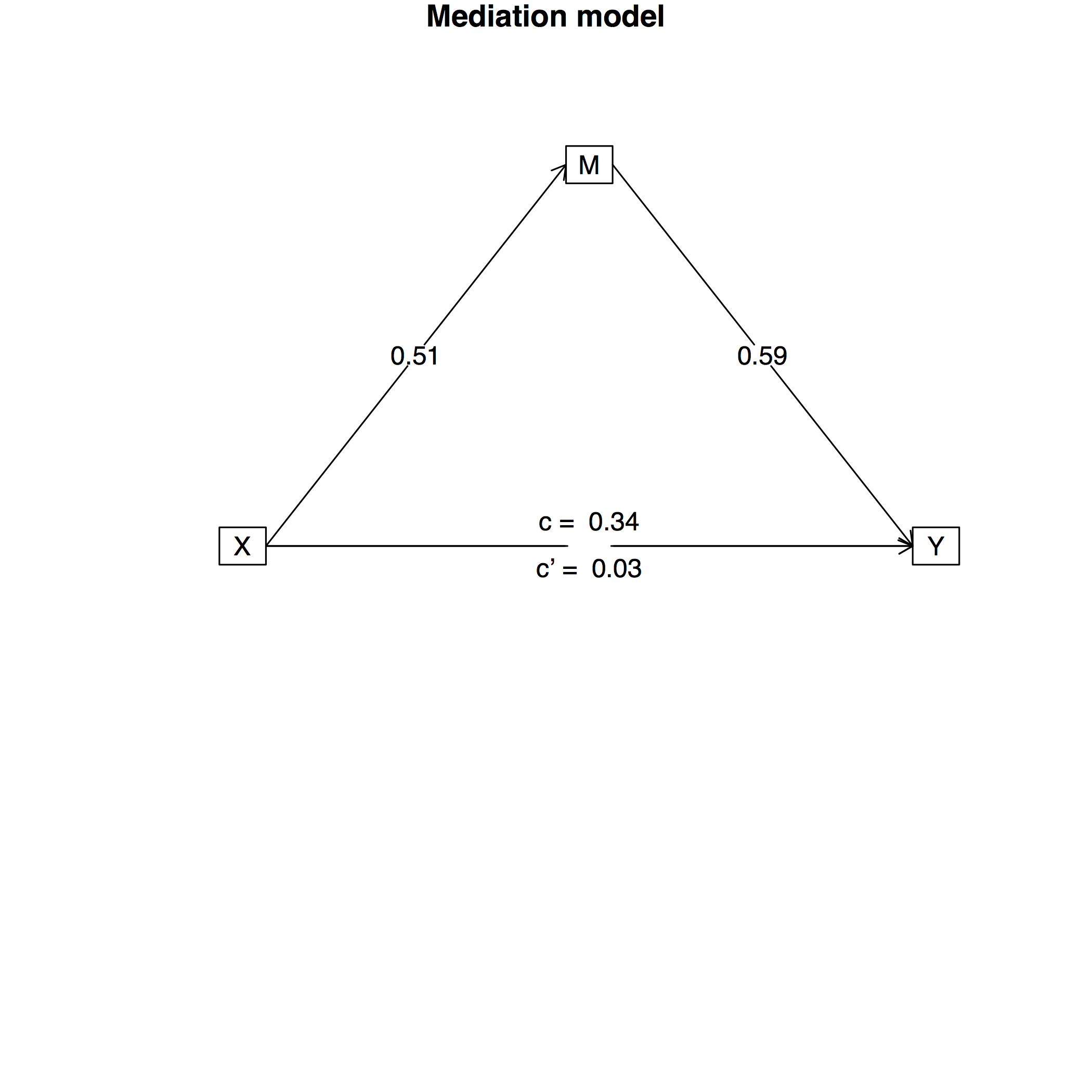
How would you report it?
Typically researchers would make a diagram as shown and then add the B or \(\beta\) coefficients. to it.
For example:

Try it yourself.
Download your dataset from here, under the data section or right click and save as here.
Conduct a causal steps mediation analysis, with math as independent variable, read as mediator and science as outcome variable.
Testing significance of the mediation.
Many ways to assess if the mediation is significant.
Older models use Sobel test. The Sobel test is also known as the ‘product’ moment approach. (Multiplication of paths). You can read also more here. There are also alternatives (Goodman / Aroian test).
Recommendation is bootstrapping methods. One method is Preacher & Hayes (2004)
Sobel test
require(bda)
# reload (note that
# Rmarkdown is
# forgetful, so you
# might want to
# reload the data)
Data_med <- read.csv("http://static.lib.virginia.edu/statlab/materials/data/mediationData.csv")
mediation.test(Data_med$M,
    Data_med$X, Data_med$Y)
##                Sobel       Aroian      Goodman
## z.value 4.327891e+00 4.299405e+00 4.356951e+00
## p.value 1.505439e-05 1.712572e-05 1.318868e-05
Sample write up.
A Sobel z test showed that the mediation effect reported in Fig. X was significant (Sobel z= 4.33, p<.0001).
Three measures.
Slight differences in calculation.
Some recommend Aroian. (I am largely indifferent, and have mostly used Sobel in my previous work).
Downside measures only work well in ‘large’ samples (opinions vary as to what large is, perhaps >100 - but when in doubt use different method).
Bootstrapping to the rescue!
Mediation
Here we use 10,000 bootstraps. The std=T command ensures standardization.
require(psych)
mediationmodel1 <- mediate("Y", "X", m = c("M"), std = TRUE,
    data = Data_med, n.iter = 10000, plot = F)
Output
Exported the results. sink() command.
sink("mediation.txt")
mediationmodel1
sink()
##
## Mediation/Moderation Analysis
## Call: mediate(y = "Y", x = "X", m = c("M"), data = Data_med, n.iter = 10000,
##     std = TRUE, plot = F)
##
## The DV (Y) was  Y . The IV (X) was  X . The mediating variable(s) =  M .
##
## Total effect(c) of  X  on  Y  =  0.34   S.E. =  0.1  t  =  3.56  df=  97   with p =  0.00057
## Direct effect (c') of  X  on  Y  removing  M  =  0.03   S.E. =  0.09  t  =  0.36  df=  97   with p =  0.72
## Indirect effect (ab) of  X  on  Y  through  M   =  0.3
## Mean bootstrapped indirect effect =  0.3  with standard error =  0.06  Lower CI =  0.19    Upper CI =  0.43
## R = 0.61 R2 = 0.37   F = 28.85 on 2 and 97 DF   p-value:  1.47e-10
##
##  To see the longer output, specify short = FALSE in the print statement or ask for the summary
Result
Click here
Sample write up:
A mediation model with 10,000 bootstraps indicated that the indirect path was significant, \(\beta\)= .3, SE = .06, 95% CI [.1, .43].
You could add the package which produced this.
Plot.
setEPS()
postscript("path.eps", horizontal = FALSE, onefile = FALSE, paper = "special")
par(mar=c(1,1,1,1))
mediate.diagram(mediationmodel1)
dev.off
Try it yourself.
Conduct either a Sobel test or a bootstrapping test for the mediation you just did.
Other method: ‘mediate’ package.
Based on this paper.
Long story short, this is a newer and perhaps better method.
Mediate
require(mediation)
med.fit <- lm(M ~ X, data = Data_med)
out.fit <- lm(Y ~ X + M, data = Data_med)
# Robust SE is ignored for Bootstrap. Otherwise
# omit boot=TRUE.
set.seed(1984)
med.out <- mediate(med.fit, out.fit, treat = "X", mediator = "M",
    boot = TRUE, sims = 10000)
Results
summary(med.out)
##
## Causal Mediation Analysis
##
## Nonparametric Bootstrap Confidence Intervals with the Percentile Method
##
##                Estimate 95% CI Lower 95% CI Upper p-value
## ACME             0.3565       0.2141         0.53  <2e-16 ***
## ADE              0.0396      -0.1962         0.30  0.7482
## Total Effect     0.3961       0.1536         0.64  0.0008 ***
## Prop. Mediated   0.9000       0.4786         2.03  0.0008 ***
## ---
## Signif. codes:  0 '***' 0.001 '**' 0.01 '*' 0.05 '.' 0.1 ' ' 1
##
## Sample Size Used: 100
##
##
## Simulations: 10000
Summary
The mediation analysis showed a significant average causal mediation effect (ACME): 0.36, 95%CI [0.21, 0.52], but the average direct effect (ADE) was not significant .04, 95%CI [-0.20, 0.30].
Plot
plot(med.out)

Sensitivity analysis
‘The sequential ignorability assumption must be satisfied in order to identify the average mediation effects. This key assumption implies that the treatment assignment is essentially random after adjusting for observed pre-treatment covariates and that the assignment of mediator values is also essentially random once both observed treatment and the same set of observed pre-treatment covariates are adjusted for.’ (Imai et al., 2011, pp. 863–864)
Simply put: no hidden or unmeasured confounder(s), accounting for what we find!
Sensitivity parameter.
Simply put, the sensitivity parameter corresponds to the correlation between errors in the step 2 and step 3 regression equations in Baron & Kenny’s terms.
It is assumed to be 0.
This parameter is denoted by \(\rho\).
Under sequential ignorability, \(\rho\) is equal to zero and thus the magnitude of this correlation coefficient represents the departure from the ignorability assumption (about the mediator).
How to test it?
sensitivity_analysis<-medsens(med.out, rho.by = 0.05)
summary(sensitivity_analysis)
##
## Mediation Sensitivity Analysis for Average Causal Mediation Effect
##
## Sensitivity Region
##
##       Rho    ACME 95% CI Lower 95% CI Upper R^2_M*R^2_Y* R^2_M~R^2_Y~
## [1,] 0.40  0.1141      -0.0016       0.2297       0.1600       0.0738
## [2,] 0.45  0.0766      -0.0357       0.1889       0.2025       0.0934
## [3,] 0.50  0.0358      -0.0742       0.1459       0.2500       0.1153
## [4,] 0.55 -0.0093      -0.1187       0.1002       0.3025       0.1395
## [5,] 0.60 -0.0601      -0.1713       0.0511       0.3600       0.1660
##
## Rho at which ACME = 0: 0.55
## R^2_M*R^2_Y* at which ACME = 0: 0.3025
## R^2_M~R^2_Y~ at which ACME = 0: 0.1395
Interpretation
\(R^2_M*R^2_Y\) the proportion of the previously unexplained variance in the mediator and outcome variables is required to be explained by an unobservable pretreatment confounder in order to render a mediation of 0.
\(\widetilde{R^2_M}\widetilde{R^2_Y}\): How much of the proportion of the original variance explained by an unobserved confounder is required to render a mediation effect of 0?
–> 0.1395 . Depending on where you stand that’s substantial or not.
Critique
Many models could fit, no evaluation in terms of absolute fit. Perhaps, a model with several main effects also fits the data well. We will return to this when we discuss SEM.
When fitting multiple mediators, those will be averaged! So, there could be a scenario where one is important but another one is not.
Exercise
Download the data ‘PSE_MOL_Doors.sav’, these are the data from an experiment by Kamila Irvine and Piers Cornelissen. This file contains data on 95 women performing various scales and body image-related tasks. doors_front is the score from a gap estimation task, w_dn is the actual gap a participant can pass through. The (estimated) Point of subjective equality or PSE (the BMI they believe themselves to be) when viewing an imageset varying in BMI. Participants used the method of adjustment to estimate their body size with the same stimulus set as for the yes-no task (MOL). BMI is the participant’s actual BMI.
Test the mediation model: doors_front –> PSE –> BMI via the causal steps method by Baron & Kenny. Report as you would do in a paper.
Make a diagram. (use ‘mediate’)
Exercise (cont’d)
Calculate a Sobel z test and report.
Test the mediation via Preacher & Hayes method.
Now test a mediation model with 2 mediators (PSE and MOL) but with the same independent and dependent variables.
Export a figure for that mediation model.
Test the mediation via Imai et al.’s method.
BONUS: perform the sensitivity analysis via Imai et al.’s method.
References (and further reading.)
Also check the reading list! (many more than listed here)
- Kim, B. (2016). Introduction to Mediation Analysis http://data.library.virginia.edu/introduction-to-mediation-analysis/
- Hayes, A. F. (2013). Introduction to Mediation, Moderation and Conditional Process Analysis. New York, New York: Guilford Press.
- Imai, K., Keele, L., & Tingley, D. (2011). A general approach to causal mediation analysis. Psychological Methods, 15(4), 309–334. https://doi.org/10.1037/a0020761
- Sobel, M. E. (1982). Asymptotic Confidence Intervals for Indirect Effects in Structural Equation Models. Sociological Methodology, 13, 290. https://doi.org/10.2307/270723